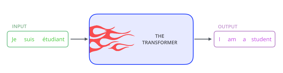
This post is a detailed explanation of the Transformer model, as described in the paper Attention is All You Need by Vaswani et al. (2017). I have tried to be concise with my mathematical notation, but if you find any errors, please let me know. This post is meant to be a reference for myself, and I hope it helps you too.

Preprocessing

Tokenization

Define the units ($U$) of your model - this can be a character, subword, word, depending on your use case.

Further, we perform a few housekeeping steps to standardize the model, including:

1. Train-test-split
2. Creating batches of size $B$ with $T$ units: $U \times 1 \implies B \times [U \times T]$
3. $X$ and $Y$ created through next-unit loops (bigram matrix)
4. Token embedding layer created: $T_{N \times E}$ is a token embedding matrix that takes in a unique list of units ($N$) and learns a $E$-dimensional vector for each
5. Positional embedding layer created: $P_{N \times E}$ is a positional embedding matrix that takes in a list of possible positions and learns a $E$-dimensional vector for each. This is necessary because the self-attention mechanism in transformers doesn't have any inherent sense of position or order of the tokens.
6. Final embedding layer: $E_{N \times E} = T + P$

Encoder layer

Attention

The self-attention mechanism allows each token to look and learn from a number of other tokens (in theory, infinitely many). Self-attention is the method the Transformer uses to bake the “understanding” of other relevant units into the unit that we are currently processing.

A single head (Query-Key-Value to Score)

The first step is to generate three vectors from each of the input vectors, which are contained in $E$.

A head size $H$ is chosen as a hyperparameter, which signifies the dimensionality of each head's output.

Three weight layers are defined,

1. Query weights ($W^Q_{E \times H}$)
2. Key weights ($W^K_{E \times H}$)
3. Value weights ($W^V_{E \times H}$)

Then, the individual vectors are created for each input $x$:

• Query: $Q = X \times W^Q$
• Key: $K = X \times W^K$
• Value $V = X \times W^V$

The second step is to calculate a score for each query and key. So, for example, $x_1$ with a query vector $q_1$ and $k_1$ will get a score vector $S_{1}$

Similarly, all $x_E$ will get their own score vector $S_{E} = Q \times K^T$

Then, divide $S$ with the square root of the head size $H$ and pass through a softmax function as:

This is then multiplied to the value vector $V$, so overall it becomes:

Multi-headed attention

Now, this can be further refined by adding multiple such heads and allowing them to communicate. This will help the model to learn about relationships between positions even more by expanding the representation subspace, i.e., projecting it to a higher dimension to capture granularity.

Thus, with $k$ number of heads, each head can independently learn the weight matrices $W_0^Q,W_0^K,W_0^V,\dots,W_k^Q,W_k^K,W_k^V$, and produce a set of scores $z_0,\dots,z_k$.

Then, the set of scores is concatenated to create a score matrix $Z$

The output of this layer is then multiplied with another weight matrix $W^O$ to produce the final output matrix

Residual pathways and LayerNorm

After the self-attention is computed, it passes through an "Add and Normalize" layer which does:

The above (pre-norm) is taken directly from the original paper. However, in Andrej Karpathy's video (YouTube), he mentions changing the formula to a more recent version:

Feed-forward layer

The model takes the self-attention for each vector $x$ in the input and passes it through a feed forward layer, which is comprised of:

1. Linear layer: $FF^1_{E \times GE}$
2. ReLU activation
3. Linear layer: $FF^2_{GE \times E}$

After this, the output passes through another add and norm layer:

Stacking

The block defined above can now be stacked $M$ times such that the outputs from one block become the inputs for next one, increasing the number of parameters available.

Once done, the output passes into the decoder layers.

Decoder layer

The first part inside a decoder layer is exactly similar to the encoder layer, with the small change of processing output vectors instead of input vectors. In other words, the decoder layer starts by taking in the outputs $Y$ and passing them through the "self-attention-feed-forward" block.

Self-attention

One key distinction in the self-attention mechanism between the encoder and decoder block lies in the treatment of future tokens. The decoder block is only allowed to attend to earlier positions in the output sequence since this would be the case during inference. This is achieved by masking the future tokens using a lower triangular matrix.

Cross-attention

For the "encoder-decoder" attention block, the idea remains the same. However, here the key and value matrices are taken as an input from the encoder block, while the query matrix is taken from the decoder block below (the one with self-attention)

Residual pathways and LayerNorm

Again, this section of the block remains the same. Each attention layer is preceded with a layer normalization and then added to the original layer via a residual connection, then sent into the feed forward layer.

Stacking

The decoder block (with self-attention and cross-attention) can be stacked together $M$ times in a similar fashion to increase the complexity of the model. The final layer will output a vector of size $E$

Final linear and softmax layer

With the output of the decoder stack, this final linear layer projects it back into a vector equal to the size of the vocabulary $N$

Then, a softmax layer normalizes the values to probabilities (all add up to 1.0) and chooses the element with the highest probability as the next output unit.'

Training

When training a model, it is important to have a function that keeps track of how well the model is performing. In other words, this means giving an objective function to the model that it should try and solve, instead of mindlessly trying to assign random values. This is called the "loss function".

Given the $X$ and $Y$ batches, the data flows through the encoder/decoder blocks and into the final softmax layer to produce a probability distribution. Since we know the actual value that should come next (from $Y$), we can compute the loss using the cross-entropy function, and instruct the model to choose the parameter weights such that the loss is minimized.

Inference

Once the model is trained using the chosen hyperparameters and an acceptable loss value, the next step is to actually use the model to generate some outputs.

This is done by giving it a starting context, and then letting the model generate outputs up to a specified number of units or some characters, depending on the use case.

Hyperparameter summary

To summarize, the non-exhaustive choice of hyperparameters when building a transformer are:

1. Vocabulary size $N$ (usually decided through the tokenization mechanism and input data)
2. Batch size $B$
3. Block size $T$
4. Number of embeddings $E$
5. Head size $H$
6. Number of heads $\frac{E}{H}$
7. Number of blocks $M$
8. Inner-layer dimensionality $GE$

Conclusion

In this post, we've explored the intricate architecture of the Transformer model, delving into the mechanics of its encoder and decoder layers, and the pivotal role of the self-attention mechanism.

As we've seen, the Transformer's ability to handle sequential data without the constraints of sequential computation, as well as its parallelization capabilities, make it a powerful tool in the machine learning toolkit. The influence is evident in the numerous models that have since been built upon its architecture (most notably GPT-3.5 and GPT-4), pushing the boundaries of what's possible in machine learning.

I've learned a lot from writing this post, and I hope you've found it useful too. If you have any questions or suggestions, please feel free to reach out to me on Twitter.

References

The following were of immense help in understanding the architecture:

1. The Illustrated Transformer – Jay Alammar – Visualizing machine learning one concept at a time.
2. Let's build GPT: from scratch, in code, spelled out. - YouTube